Timeseries classification with CNN and Embeddings


from common import *
from config import *
from dataloaders import *
from transform_data import *
from model_part import *
from callbacks import *

from functools import partial
from scipy.io import arff
import matplotlib.pyplot as plt
# Read data
data_train = arff.loadarff('data/LargeKitchenAppliances_TRAIN.arff')
data_test = arff.loadarff('data/LargeKitchenAppliances_TEST.arff')
df_test = pd.DataFrame(data_test[0])
df_train = pd.DataFrame(data_train[0])

# let's add a categorical variable
countries = ['Germany', 'US']
household_income = ['low', 'high']
df_train["country"] = np.random.choice(countries, len(df_train))
df_test["country"] = np.random.choice(countries, len(df_test))
df_train["household_income"] = np.random.choice(household_income, len(df_train))
df_test["household_income"] = np.random.choice(household_income, len(df_test))

df_train.head()
df_train.shape, df_test.shape
The first 720 columns represent the time-dependent variables, the second last is our target_variable and the last is our (fake) categorical variable.
x_train = df_train.iloc[:, :-3].values.reshape(-1, 1, 720)
x_test = df_test.iloc[:, :-3].values.reshape(-1, 1, 720)

y_train = df_train.iloc[:, -3].values
y_test = df_test.iloc[:, -3].values

emb_vars_train = df_train.iloc[:, -2:].values
emb_vars_test = df_test.iloc[:, -2:].values
Let's plot some of these:
df_train.iloc[0, :-3].plot.line(title=f'time series with class = {df_train.iloc[0, -3]} in {df_train.iloc[0, -2]}');

df_train.iloc[10, :-3].plot.line(title=f'time series with class = {df_train.iloc[10, -3]} in {df_train.iloc[10, -2]}');

Let's check the means and variance of our variables:
plt.plot(x_train.mean(axis=2).reshape(-1))

plt.plot(x_train.var(axis=2).reshape(-1))

Note the 1e-8 on top, meaning we're dealing here with numbers almost being 0 for the mean and almost being 1 for the variance, so we do not need to normalize them, because they already are. Still, I want to show you a neat trick of how to use broadcasting to quickly normalize each column to have mean of zero and variance of 1:
def normalize(x, m, s): return (x-m)/s

means_ = x_train.mean(axis=2)
vars_ = x_train.var(axis=2)
means_.shape, vars_.shape, x_train.shape
Only the last dimensions does not match, therefore we can use broadcasting to normalize over all columns:
normalize(x_train, means_, vars_).shape
Again, in this case our data already looks as it should. Also, the kind of function like normalize I put into a .py file with the name common, which can then be imported by any other python-file or notebook, just as I did right on top of this notebook. So whenever in this notebook there appears a function which is not defined so far, look into the common.py file.
As a next step, we need to transform the target variable and the categorical variable into something the computer can actuelly work with, meaning a number. We can do this using the cat_transform function:
y_train, y_test, dict_y, dict_inv_y = cat_transform(y_train, y_test)
emb_vars_train, emb_vars_test, dict_embs, dict_inv_embs = cat_transform(emb_vars_train, emb_vars_test)
y_train[:10], emb_vars_train[:10], dict_y, dict_embs
dict_y, dict_embs
Next, we will use PyTorch to create dataset and dataloader, which we will put into a class called DataBunch (idea stolen from fastai).
device = DEVICE
datasets = create_datasets(x_train, emb_vars_train, y_train,
             x_test, emb_vars_test, y_test,
             valid_pct=VAL_SIZE, seed=1234)
data = DataBunch(*create_loaders(datasets, bs=1024))
Next, we define our model. First, we need to make sure that the final convolution ends up with 1 as the last dimension, so we can put it through a linear layer.
# define model
raw_feat = x_train.shape[1]
emb_dims = [(len(dict_embs[0]), EMB_DIMS), (len(dict_embs[1]), EMB_DIMS)]

num_classes = len(dict_y[0])
Let's grab a batch from our data and see how the convolutions work on our timeseries data:
x_raw, _, _ = next(iter(data.train_dl))
x_raw.shape
raw_ni=x_train.shape[1] # no of input features (here:1)
drop=0.3
m = nn.Conv1d(raw_ni, 128, 28, 7, 0)
output_ = m(x_raw)
print(output_.shape)
m = nn.Conv1d(128, 32, 14, 7, 0)
output_ = m(output_)
print(output_.shape)
m = nn.Conv1d(32, 64, 5, 2, 0)
output_ = m(output_)
print(output_.shape)
# m = nn.Conv1d(64, 32, 3, 8, 0)
# output_ = m(output_)
# print(output_.shape)
m = nn.MaxPool1d(2, stride=4)
output_ = m(output_)
print(output_.shape)
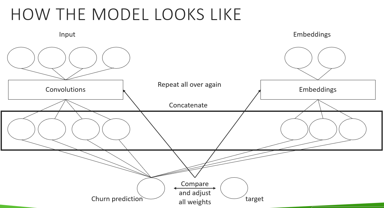
To easily try different kind of architectures, I created a helper function which creates the CNN part of our model. How the complete architecture works will be part of the following tutorial, where I will show in more detail how the code works. But for now, let's see how the final architecture of the model looks like:
output_shapes = [128, 32, 64]
kernels_shape = [28, 14, 5]
strides = [7, 7, 2]

model = Classifier_CNN(nn.Sequential(
    *get_cnn_layers(raw_feat, output_shapes, kernels_shape, strides)
    ), emb_dims, num_classes).to(device)
opt = optim.Adam(model.parameters(), lr=0.01)
loss_func = nn.CrossEntropyLoss()
This is how the CNN-Part from our model looks like:
model.raw
And this is how the embedding part looks like:
model.embeddings
A pretty neat technique of how to enhance a class with different behaviour is called a Callback. For example, we can use a function to calculate the best learning rate, and use a Callback to use our model with it. Again, how this exactly works will be covered in the next tutorial:
learn = Learner(model, opt, loss_func, data)
run = Runner(cb_funcs=[LR_Find, Recorder])
run.fit(1000, learn)
run.recorder.plot(skip_last=5)

We should take the learning rate with the steepest drop, so somewhere between 1e-3 and 1e-2.
model = Classifier_CNN(nn.Sequential(
    *get_cnn_layers(raw_feat, output_shapes, kernels_shape, strides)
    ), emb_dims, num_classes).to(device)
opt = optim.Adam(model.parameters(), lr=2e-2)
cbfs = [Recorder, partial(AvgStatsCallback,adjusted_accu)]
learn = Learner(model, opt, loss_func, data)
run = Runner(cb_funcs=cbfs)
run.fit(50, learn)
Even though this specific model didn't turn out to be too good, being correct in only approximately 60% of the time (there are 3 classes of which to choose), you can see how I again used a Callback to forward a metric which showed here as the accuracy.
run.recorder.plot_loss()

Next to the validation set I also use the testset to check how good our predictions actually are.
outs = run.predict(learn, learn.data.test_dl)
outs[:10]
(outs == y_test).mean()
run.predict_metrics(learn, learn.data.test_dl, list(dict_y[0].values()))

We're pretty good at identifying class b1, however the model completely fails when it comes to classifying b2.
df_test.iloc[0, :-3].plot.line(title=f'time series with class = {df_test.iloc[0, -3]}, predicted to be class {outs[0]}');

df_test.iloc[10, :-3].plot.line(title=f'time series with class = {df_test.iloc[10, -3]}, predicted to be class {outs[10]}');

df_test.iloc[8, :-3].plot.line(title=f'time series with class = {df_test.iloc[8, -3]}, predicted to be class {outs[8]}');

df_test.iloc[57, :-3].plot.line(title=f'time series with class = {df_test.iloc[57, -3]}, predicted to be class {outs[57]}');

df_test.iloc[326, :-3].plot.line(title=f'time series with class = {df_test.iloc[326, -3]}, predicted to be class {outs[326]}');

Also one particular interesting measure is to look inside the model, meaning having a look at the means and standard-deviations of our activations. ideally the mean should be around 0 and the standard-variance about 1.
def append_stats(i, mod, inp, outp):
    act_means[i].append(outp.data.mean())
    act_stds [i].append(outp.data.std())
output_shapes = [128, 32, 64]
kernels_shape = [28, 14, 5]
strides = [7, 7, 2]

model = Classifier_CNN(nn.Sequential(
    *get_cnn_layers(raw_feat, output_shapes, kernels_shape, strides)
    ), emb_dims, num_classes).to(device)

model.raw[0][0].register_forward_hook(partial(append_stats, 0))
model.raw[1][0].register_forward_hook(partial(append_stats, 1))
model.raw[2][0].register_forward_hook(partial(append_stats, 2))

cbfs = [Recorder]
learn = Learner(model, opt, loss_func, data)
run = Runner(cb_funcs=cbfs)

act_means = [[] for _ in range(3)]
act_stds  = [[] for _ in range(3)]

run.fit(50, learn)
for o in act_means: plt.plot(o)
plt.legend(range(3));

for o in act_stds: plt.plot(o)
plt.legend(range(3));

This is really interesting, this zigzag pattern in the later layers meaning we're actually not learning really well here. Let's try another, much simpler architecture and compare the results:
output_shapes = [128]
kernels_shape = [719]
strides = [1]

model = Classifier_CNN(nn.Sequential(
    *get_cnn_layers(raw_feat, output_shapes, kernels_shape, strides)
    ), emb_dims, num_classes).to(device)
opt = optim.Adam(model.parameters(), lr=0.001)
cbfs = [Recorder]
learn = Learner(model, opt, loss_func, data)
run = Runner(cb_funcs=cbfs)

act_means = [[] for _ in range(1)]
act_stds  = [[] for _ in range(1)]

model.raw[0][0].register_forward_hook(partial(append_stats, 0))

run.fit(50, learn)
for o in act_means: plt.plot(o)
plt.legend(range(1));

for o in act_stds: plt.plot(o)
plt.legend(range(1));

This looks better. However, we can also try a different initilization.
def init_weights(m):
    if isinstance(m, nn.Conv1d):
        torch.nn.init.kaiming_uniform_(m.weight)
        m.bias.data.fill_(0.01)
output_shapes = [128, 32, 64]
kernels_shape = [28, 14, 5]
strides = [7, 7, 2]

model = Classifier_CNN(nn.Sequential(
    *get_cnn_layers(raw_feat, output_shapes, kernels_shape, strides)
    ), emb_dims, num_classes).to(device)

model.apply(init_weights)

model.raw[0][0].register_forward_hook(partial(append_stats, 0))
model.raw[1][0].register_forward_hook(partial(append_stats, 1))
model.raw[2][0].register_forward_hook(partial(append_stats, 2))

cbfs = [Recorder]
learn = Learner(model, opt, loss_func, data)
run = Runner(cb_funcs=cbfs)

act_means = [[] for _ in range(3)]
act_stds  = [[] for _ in range(3)]

run.fit(50, learn)
for o in act_means: plt.plot(o)
plt.legend(range(3));

for o in act_stds: plt.plot(o)
plt.legend(range(3));

This looks way more promising when it comes to the 3 convolutional layers. Admittingly, this still is not perfect.
model = Classifier_CNN(nn.Sequential(
    *get_cnn_layers(raw_feat, output_shapes, kernels_shape, strides)
    ), emb_dims, num_classes).to(device)

model.apply(init_weights)

opt = optim.Adam(model.parameters(), lr=2e-2)
cbfs = [Recorder, partial(AvgStatsCallback,adjusted_accu)]
learn = Learner(model, opt, loss_func, data)
run = Runner(cb_funcs=cbfs)
run.fit(80, learn)
outs = run.predict(learn, learn.data.test_dl)
(outs == y_test).mean()
This is the end of the first part of this tutorial. In the next tutorial I will show you how the code behind this looks like and how it works.
Lasse